Machine learning models learn dependencies between inputs and labels from the training set during training. However, dependency does not always imply the causality that we really want to learn. This becomes a problem when the data distribution of production differs from the data distribution of the training set. Then, the learnt dependency between input and ground truth label may disappear if there was not a real causality in the first place. This dependency may be generated by some hidden mechanisms, or it may be pure random effect in the training data set. From the former case one often talks about AI bias that can lead to discriminating decisions. The latter case is related to overfitting.

The former case has been identified as a problem for a long time ago. Therefore, certain level of transparency and explainability of machine learning decisions are required even in EU regulations for fighting against discriminating machine learning systems.

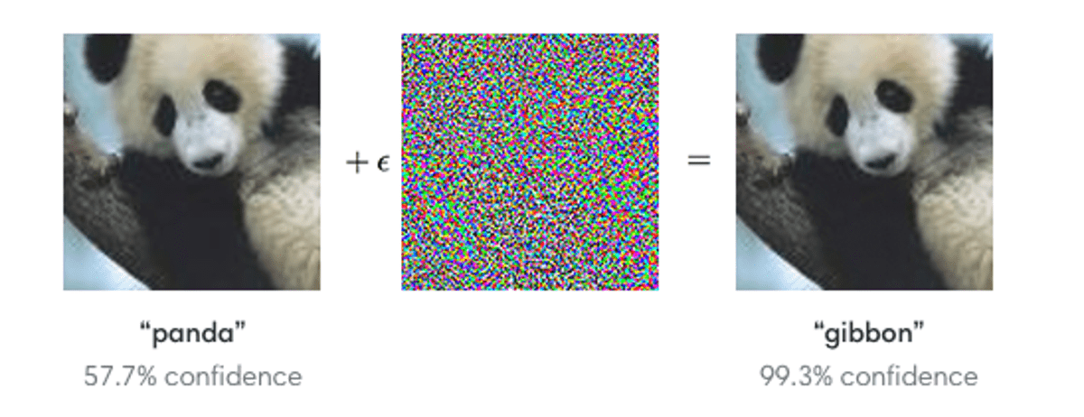
The latter more random mechanism is interesting as well. There have been well working image classification systems when tested with limited data sets. However, when changing just one well-chosen pixel in input image, the classifier starts to make completely wrong decisions. In this case there have been some random dependencies in training data inputs and outputs that the machine has learnt. Check this for details [1]. However, more classical demonstration of this issue is given by Goodfellow et al [2], also shown in below figure, where instead of one manipulated pixel, tiny well-chosen noise is added to the whole image that confuses GoogLeNet image classification model.

At Talenom we have developed machine learning based invoice posting system. To develop a state-of-the-art machine learning system, we want to ensure that machine has learnt the right causal logic instead of other dependencies to ensure that our machine works well for new kind of unseen invoices as well. This is important for machine learning developers and for business also. When the machine makes independent decisions at large scale, we must be able to rely on its logic.

Explainability terminology

Explainability of machine learning models is divided usually to global and local explainability. Local explainabilty is concerned for explaining a single prediction while global explainability focuses to model overall predictions. Another terminology issue is interpretability vs explainability. Usually, interpretability focuses on finding cause end effect of machine learning models while explainability is a broader concept finding also more detailed logic how the machine has concluded to its outcome. Although the methods presented here can be considered as interpretability methods, we use anyway more common term explainability since our goal is to go beyond interpretability.

Explainability methods

There exists variety of different explainability methods. We are currently using Kernel SHAP method that is a kind of combination of LIME with Shapley values [3]. In LIME method, multiple points are fed to the model that are sampled around the input sample we are interested of. These sampled points around the point of interest means that some subset of the inputs are replaced by a neutral value. However, it is not always a trivial case to define what is the proper neutral value for each input. Anyway, now we have multiple outputs for different combinations of inputs. From these we need to figure out how each input contribute to the output. This is where LIME and Kernel SHAP differ from each other. In both methods, a simple linear fit of input variable importance’s is made around the point of interest. LIME method performs this using basic linear regression while Kernel SHAP method is based on Shapley values.

The Shapley values was originally developed by Lloyd Shapley in the 50’s as a solution to the game theoretic problem of assigning players a fair reward based on their contributions to a given task, when all the information we have is who was playing and what was the outcome. The logic is that poor players reduce the performance of the whole group while good players are likely to increase it and therefore by measuring the performance of different combinations of players, we can estimate the average contributions of each individual. Now if we replace players with the inputs of a machine learning model and the performance score with the predicted output value, we have a way to measure each input’s contribution to the output.

The benefits of the Shapley values are their easy applicability to any type of machine learning algorithm and their relatively simple interpretation. Downsides exist as well and one of them is that the calculation of the Shapley values can be computationally expensive and requires at least many hundreds and preferably thousands of runs of the machine learning model.

Explainability in practice

As there are many explainability methods there are many use cases as well. Here we show two typical use case examples that are based on SHAP. One comes from image recognition domain and one from our own toolbox.

Example 1

The above images provide explanation for why the algorithm thinks the leftmost picture is of a meerkat and not of a mongoose. The algorithm has found that the distinctive dark areas around the subject’s eyes are indicative of the species as highlighted by the red color in the middle figure and not found in mongeese as shown by the blue areas in the figure on the right. This increases our confidence that the algorithm has learned to look for the correct clues in the images. The images are copied from https://github.com/slundberg/shap.

Example 2

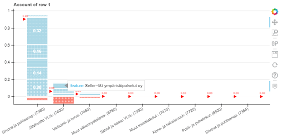
The above figure shows the explanation of the posting decision made for a single invoice. The most probable accounts for the invoice are displayed in the x-axis while each segment in the bars corresponds to the Shapley value given to one of the inputs of the model, blue denoting positive values and red negative values. For instance, the fact that the invoice was sent by company whose main business is waste management increased probability of waste management account. The sum of the positive and the negative Shapley values gives the total predicted probability (0.90) for the right account (cleaning and sanitation), shown by the little red arrow. The second most likely account is the waste management with total probability 0.06. These values give us an idea of what inputs affected the model's decision the most and help us identify cases where further developments are in order. For instance, we could find that the algorithm has learnt a shortcut that applies in the training data but is not viable in the larger context.

Usage of explanations

We have implemented an explanation endpoint for our invoice posting API. From request we can ask explanation for given invoice posting.

We go regularly though errors made by machine learning model in production using our production monitoring UI. For the interesting errors we request explanations and check why the machine learning model has made its decision with this UI. However, we have noted that although SHAP explanations are made easily interpreted, they still can sometime be misleading. Therefore, occasionally it is good to manually change some inputs to see their effect to output to get good understanding of model behavior for certain case.

We at Talenom have taken the first steps to incorporate explainable AI into our machine learning toolbox and look to develop it further as new technologies emerge. Looking deeper into the natural language contained in the invoices on word and sentence level would be one possible next step towards this direction. We also follow development of external AI explainability tools and services and their applicability to our workflow such as Google’s What-if Tool.

References

[1] Su, Jiawei & Vargas, Danilo & Sakurai, Kouichi. (2017). One Pixel Attack for Fooling Deep Neural Networks. IEEE Transactions on Evolutionary Computation. PP. 10.1109/TEVC.2019.2890858.

[2] I. J. Goodfellow, J. Shlens, and C. Szegedy, Explaining and harnessing adversarial examples, arXiv preprint arXiv:1412.6572, 2014

[3] Scott M. Lundberg and Su-In Lee. 2017. A unified approach to interpreting model predictions. In Proceedings of the 31st International Conference on Neural Information Processing Systems (NIPS'17). Curran Associates Inc., Red Hook, NY, USA, 4768–4777.